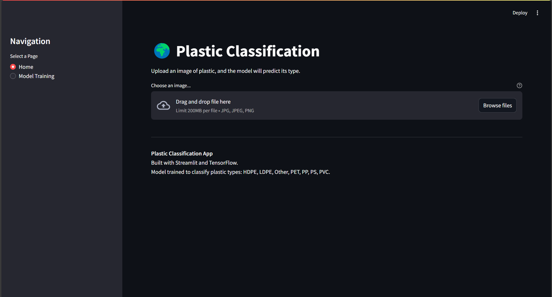
Plastic Classification using Transfer Learning

In this blog post, we will walk through the process of building a deep learning model to classify different types of plastic using Transfer Learning with TensorFlow. We will use a pre-trained MobileNetV2 model and fine-tune it for our specific task. The goal is to classify plastic images into one of seven categories: HDPE, LDPE, Other, PET, PP, PS, PVC.

Introduction
Dataset Preparation
Model Building
Training the Model
Model Evaluation
Visualizing Results
Conclusion

Introduction

Plastic classification is an important task in recycling and waste management. Automating this process using deep learning can significantly improve efficiency. In this project, we leverage Transfer Learning to build a model that can classify different types of plastic based on images.

Why Transfer Learning?

Transfer Learning allows us to use a pre-trained model (trained on a large dataset like ImageNet) and fine-tune it for our specific task. This approach is beneficial when we have a limited dataset, as it helps in achieving good performance without requiring a massive amount of data.

Dataset Preparation

Dataset Overview

The dataset consists of images of plastic items from seven different classes:

HDPE (High-Density Polyethylene)
LDPE (Low-Density Polyethylene)
Other
PET (Polyethylene Terephthalate)
PP (Polypropylene)
PS (Polystyrene)
PVC (Polyvinyl Chloride)

The dataset is split into three parts:

Training set: 1,270 images
Validation set: 354 images
Test set: 187 images

Data Augmentation

To improve the model’s ability to generalize, we apply data augmentation to the training set. This includes:

Random rotation
Width/height shifts
Shearing
Zooming
Horizontal flipping

train_datagen = tf.keras.preprocessing.image.ImageDataGenerator(
    rescale=1./255,
    rotation_range=20,
    width_shift_range=0.2,
    height_shift_range=0.2,
    shear_range=0.2,
    zoom_range=0.2,
    horizontal_flip=True,
    fill_mode='nearest'
)

Data Generators

We use TensorFlow’s ImageDataGenerator to create data generators for training, validation, and testing.

train_generator = train_datagen.flow_from_directory(
    train_dir,
    target_size=IMG_SIZE,
    batch_size=BATCH_SIZE,
    class_mode='categorical',
    shuffle=True
)

val_generator = test_val_datagen.flow_from_directory(
    val_dir,
    target_size=IMG_SIZE,
    batch_size=BATCH_SIZE,
    class_mode='categorical',
    shuffle=False
)

test_generator = test_val_datagen.flow_from_directory(
    test_dir,
    target_size=IMG_SIZE,
    batch_size=BATCH_SIZE,
    class_mode='categorical',
    shuffle=False
)

Model Building

Transfer Learning with MobileNetV2

We use MobileNetV2 as the base model for transfer learning. MobileNetV2 is a lightweight and efficient model that is well-suited for mobile and embedded vision applications.

def build_model():
    base_model = applications.MobileNetV2(
        input_shape=INPUT_SHAPE,
        include_top=False,
        weights='imagenet'
    )

    base_model.trainable = False

    inputs = tf.keras.Input(shape=INPUT_SHAPE)
    x = base_model(inputs, training=False)
    x = layers.GlobalAveragePooling2D()(x)
    x = layers.Dropout(0.2)(x)
    x = layers.Dense(128, activation='relu')(x)
    outputs = layers.Dense(NUM_CLASSES, activation='softmax')(x)

    model = models.Model(inputs, outputs)

    return model

Model Summary

The model consists of:

Base Model: MobileNetV2 (pre-trained on ImageNet)
GlobalAveragePooling2D: To reduce dimensionality.
Dropout (0.2): To prevent overfitting.
Dense (128 units): Fully connected layer with ReLU activation.
Dense (7 units): Output layer with softmax activation for multi-class classification.

model.summary()

Training the Model

Compilation

We compile the model using the Adam optimizer with an exponential learning rate decay.

initial_learning_rate = 1e-4
lr_schedule = tf.keras.optimizers.schedules.ExponentialDecay(
    initial_learning_rate,
    decay_steps=100,
    decay_rate=0.96,
    staircase=True
)

model.compile(
    optimizer=tf.keras.optimizers.Adam(learning_rate=lr_schedule),
    loss='categorical_crossentropy',
    metrics=['accuracy']
)

Callbacks

We use Early Stopping and Model Checkpoint callbacks to prevent overfitting and save the best model.

early_stopping = callbacks.EarlyStopping(
    monitor='val_loss',
    patience=10,
    restore_best_weights=True
)

model_checkpoint = callbacks.ModelCheckpoint(
    'best_model.h5',
    save_best_only=True,
    monitor='val_accuracy',
    mode='max'
)

Training

The model is trained for 50 epochs.

history = model.fit(
    train_generator,
    epochs=EPOCHS,
    validation_data=val_generator,
    callbacks=[early_stopping, model_checkpoint, tensorboard_callback]
)

Model Evaluation

Test Accuracy

After training, we evaluate the model on the test set.

test_loss, test_acc = model.evaluate(test_generator)
print(f"\nTest accuracy: {test_acc:.2%}")
print(f"Test loss: {test_loss:.4f}")

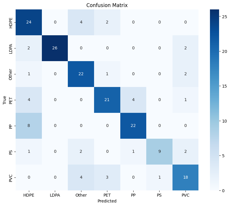
Confusion Matrix

We plot the confusion matrix to visualize the model’s performance.

def plot_confusion_matrix():
    test_generator.reset()
    predictions = model.predict(test_generator)
    predicted_classes = np.argmax(predictions, axis=1)

    cm = confusion_matrix(test_generator.classes, predicted_classes)
    plt.figure(figsize=(10, 8))
    sns.heatmap(cm, annot=True, fmt='d', cmap='Blues',
                xticklabels=class_names,
                yticklabels=class_names)
    plt.xlabel('Predicted')
    plt.ylabel('True')
    plt.title('Confusion Matrix')
    plt.show()

plot_confusion_matrix()

Visualizing Results

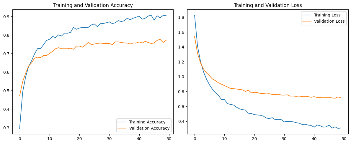
Training History

We plot the training and validation accuracy and loss to understand the model’s learning process.

def plot_history(history):
    acc = history.history['accuracy']
    val_acc = history.history['val_accuracy']
    loss = history.history['loss']
    val_loss = history.history['val_loss']

    epochs_range = range(len(acc))

    plt.figure(figsize=(12, 5))

    plt.subplot(1, 2, 1)
    plt.plot(epochs_range, acc, label='Training Accuracy')
    plt.plot(epochs_range, val_acc, label='Validation Accuracy')
    plt.legend(loc='lower right')
    plt.title('Training and Validation Accuracy')

    plt.subplot(1, 2, 2)
    plt.plot(epochs_range, loss, label='Training Loss')
    plt.plot(epochs_range, val_loss, label='Validation Loss')
    plt.legend(loc='upper right')
    plt.title('Training and Validation Loss')

    plt.tight_layout()
    plt.show()

plot_history(history)

Training Accuracy & Loss Graph

Accuracy and Loss

Confusion Matrix

Conclusion

In this project, we successfully built a deep learning model to classify different types of plastic using Transfer Learning with MobileNetV2. The model achieved a test accuracy of 75.94%, which is a good starting point for further improvements.

Future Work

Data Augmentation: Experiment with more advanced augmentation techniques.
Model Tuning: Fine-tune the hyperparameters for better performance.
Larger Dataset: Collect more data to improve the model’s accuracy.

References

This blog post provides a step-by-step guide to building a plastic classification model using Transfer Learning. The code and explanations are designed to be easy to follow, even for beginners. Feel free to explore the GitHub repository for the complete code and dataset.

Plastic Classification using Transfer Learning